
GUM based steps to compute calibration uncertainty, a three contributor worked example, and quick certificate checks including CMC verification.

Calibration uncertainty is the quantified doubt attached to a measurement result, reported as an expanded uncertainty alongside the value itself, written as y ± U at a stated coverage probability. The GUM (JCGM 100) sets the convention, typically 95% coverage with a coverage factor of k=2. When a certificate lands on your desk, check that U is stated with its k value, and if anything looks off, ask a provider like PCS Precision to verify it.
TL;DR:
- The calibration uncertainty should always be reported as an expanded uncertainty with a clearly stated coverage factor and probability, not just a numerical figure.
- It is essential to verify that the reported uncertainty does not fall below the calibration and measurement capability listed in the lab’s accreditation scope.
- The calculation involves summing the squares of individual uncertainty contributors, then applying the coverage factor to determine the expanded uncertainty.
- Proper uncertainty budgets must consider all relevant factors, including measurement repeatability, resolution, and known process limitations, avoiding common mistakes like misapplying resolution conversions.
- Prioritize checking the lab’s calibration and CMC before examining the detailed budget to ensure the uncertainty claim aligns with the lab’s accredited competence and standards.
The GUM defines measurement uncertainty as a parameter that characterises the dispersion of values that could reasonably be attributed to whatever you’re measuring, based on the available state of knowledge. That phrase matters. Uncertainty isn’t a mistake you made. It’s an honest statement of how much confidence you can place in a result, given everything from the reference standard’s own limitations to the resolution of your instrument’s display.
Dispersion is different from instrument error. Error is a specific, often correctable deviation between an indicated value and the true value. Uncertainty is the range of doubt that remains once you’ve accounted for everything you know, and everything you can’t fully pin down.
This distinction has real weight on the shop floor:
Recent literature has debated how uncertainty should be conceptually framed going forward, but for day-to-day calibration work, the operational GUM steps remain the practical standard.
No, and mixing the two up causes real compliance problems. Calibration error is an observed, specific deviation, and it usually falls into one of four categories:
Errors get identified and often corrected during calibration. Uncertainty is what’s left over: the doubt that remains even after correction. A pass/fail decision that ignores uncertainty isn’t valid, because a result sitting right on a tolerance boundary could genuinely be inside or outside spec depending on where the true value actually falls within that uncertainty band.
Every calibration certificate you review should trace back to a consistent set of standards. The core documents are the GUM (JCGM 100) for the fundamental method, JCGM 101 for Monte Carlo propagation, ISO/IEC 17025 for laboratory competence, and ILAC and Working Group on Force and Flow (WGFF) policy documents that govern how accredited labs express their capability.
Traceability means a chain of comparisons links your instrument back to a national or international standard, with uncertainty carried at every step. In practice, this shows up as a lab’s Calibration and Measurement Capability, or CMC, listed in its scope of accreditation. A lab genuinely cannot report an uncertainty smaller than its own CMC at that measurement point, no matter how good the specific job looked on the day.
Pro Tip: Before you accept any certificate, find the lab’s CMC entry for that parameter and range on their accreditation scope. If the reported uncertainty is suspiciously tighter than the CMC, ask questions before you sign off.
The calculation itself isn’t complicated once you’ve built the budget. It’s arithmetic, and it’s the kind of arithmetic you can run in a spreadsheet in a few minutes.
Here’s a worked example for a digital force gauge calibrated at 500 N, with three contributors identified.
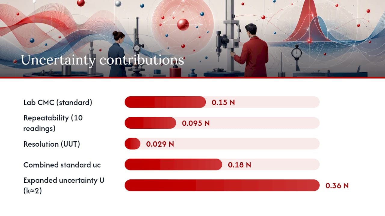
Contributor 1, the lab’s CMC at this range is stated as 0.15 N (already a standard uncertainty from the calibrating lab’s own accreditation scope).
Contributor 2, repeatability of the unit under test (UUT) across 10 readings gives a standard deviation of 0.30 N. Divided by √10, that’s a standard uncertainty of 0.095 N.
Contributor 3, UUT resolution is 0.1 N. Divided by 2√3, that’s a standard uncertainty of 0.029 N.
Squaring and summing these: 0.15² + 0.095² + 0.029² = 0.0225 + 0.009 + 0.0008 = 0.0323.
The square root gives a combined standard uncertainty (uc) of approximately 0.18 N.
Applying an appropriate coverage factor (commonly around 2) for approximately 95% coverage probability gives the expanded uncertainty.
That’s the entire calculation, start to finish, using three contributors and basic RSS combination. Where a measurement model is genuinely non-linear, or an input distribution is far from normal, the GUM’s standard linear propagation starts to break down. That’s when Monte Carlo propagation, described in JCGM 101, becomes the better tool. NIST’s Uncertainty Machine implements exactly this, letting you run a full propagation-of-distributions calculation without building the maths from scratch. It’s also worth knowing that calibration curves add a layer of complexity: uncertainty from limited calibration data combines with the uncertainty of a future measurement, and that combination sometimes needs special formulae of its own.
A certificate that hides its uncertainty convention isn’t giving you the full picture. Reporting should always follow y ± U notation, with the coverage factor k and coverage probability stated in the same breath, either as an absolute value in measurement units or, for wide-ranging instruments, as a relative percentage.
Rounding matters more than most technicians assume. The convention is two significant digits for U, with the final result rounded to match the same decimal place as the uncertainty figure.
Before you accept any certificate, check that it states:
Miss any of these fields, and the certificate is arguably incomplete, whatever the numbers say.
The same handful of errors show up again and again on certificates and in internal calibration records:
Run a quick check: does the reported U sit at or above the CMC? Are contributors listed individually, not just as one bundled number? Is k stated, not implied?
Pro Tip: Always record as-found and as-left values for every calibration, not just the final adjusted result. That paired record is what lets you spot drift trends over successive calibration cycles, long before a unit fails outright.
PCS Precision has spent decades delivering NATA-accredited calibration across manufacturing, laboratory, food, pharmaceutical, and aerospace sectors, and that hands-on experience with certificates, CMC scopes, and instrument behaviour underpins the method described here. This guide draws on PCS Precision’s ongoing calibration blog contributions from author Nima, alongside the GUM and ILAC framework referenced throughout.
If you want to check how accreditation scope and CMC actually appear on a certificate, PCS Precision’s guide to NATA calibration standards walks through it in more depth, and the piece on digital calibration certificates covers how modern reporting formats present uncertainty data.
Most guidance on calibration uncertainty spends its energy on the maths and almost none on the judgement calls that actually determine whether a budget is any good. The RSS calculation is genuinely simple, a spreadsheet exercise. What’s underrated is knowing which contributors to even include, and that comes from understanding your specific instrument and process, not from a formula.
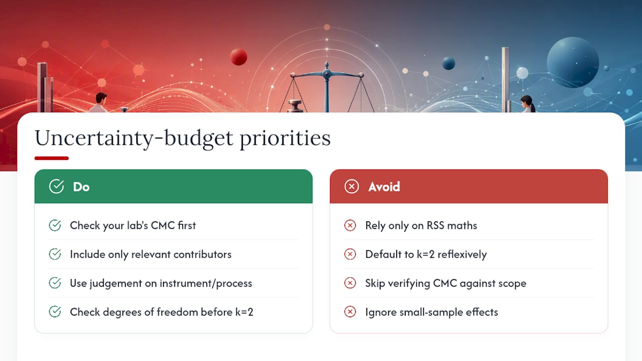
The industry also leans too hard on k=2 as a reflex. It’s the right choice for large sample sizes and normal distributions, but plenty of calibration jobs involve small repeatability sets where the Welch-Satterthwaite approach genuinely changes the coverage factor. Defaulting to k=2 without checking degrees of freedom is a shortcut that occasionally gets the reported uncertainty wrong.
If there’s one priority for a QA team building its first proper uncertainty budget, it’s this: check your lab’s CMC before you build anything else. Every other contributor sits on top of that floor, and no amount of careful repeatability analysis fixes a budget built on a CMC figure nobody actually verified against the accreditation scope.
— Nima
Accredited calibration work typically includes certificates stating expanded uncertainty, coverage factor, and coverage probability in accordance with GUM guidelines. Whether calibration is performed on-site or in-house, the process generally includes a documented uncertainty budget suitable for audit purposes.
If a current certificate lacks detail, it is advisable to confirm the CMC for your instrument’s range before relying on it for a pass/fail decision. For labs weighing up new equipment alongside their next calibration cycle, instruments like the Ohaus Aquasearcher AB33M1 Bench Meter are worth reviewing against your own uncertainty requirements before purchase. Get in touch through PCS Precision to request an uncertainty budget or book your next calibration appointment.
A useful uncertainty budget lists every contributor separately before combining anything. The usual suspects are:
These split into two evaluation types under the GUM. Type A evaluation uses statistical analysis of repeated observations, usually a standard deviation. Type B evaluation covers everything else: manufacturer specifications, calibration certificates, or engineering judgement.
Converting these into standard uncertainty follows well established shortcuts. Resolution, treated as a rectangular distribution, is divided by 2√3. Repeatability, evaluated across multiple readings, is divided by the square root of the number of readings to get the standard uncertainty of the mean.
